Drivers of Climate
Earth’s Energy Balance
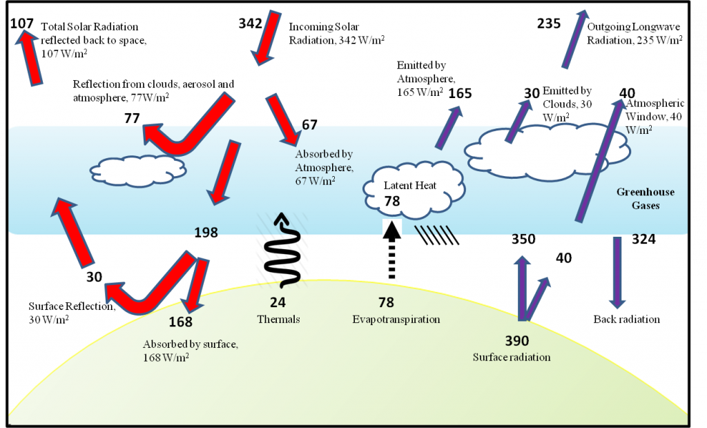
Figure 1. Annual energy budget of the earth (global mean) (Kiehl and Trenberth, 1996).
Basically, the earth’s climate is the outcome of a balance between the incoming solar radiation and the outgoing radiation from the earth’s atmosphere and surface. In order to keep this balance, a complex interaction happens between different components of climate system (Kiehl and Trenberth, 1996). Such interaction involves processes of absorption and reflection of shortwave radiation, emission of longwave radiation, and the exchange of heat energy between the earth’s surface and its atmosphere through the processes of evaporation, condensation, and convection (Figure 1). The annual balance shown in the above figure is averaged over entire globe. Practically, such energy balance at any place on the earth’s surface is being governed by the latitude, longitude and season of the year.
From the above figure, one can verify the balance between outgoing and incoming radiation at various levels like at the top of the atmosphere, or at the surface. In a balanced situation, mean climate of the earth remains unchanged. Changes into any of these climate components will perturb this balance causing various interactions and processes to adjust accordingly in order to achieve a new energy balance, and this would lead to climate change. This change in the energy balance (net energy flux into the climate system) is being termed as a radiative forcing of climate (IPCC, 2013). For example, if there is an increase in the concentration of greenhouse gases (GHGs) (carbon dioxide (CO2), methane (CH4), water vapour (H2O), ozone (O3), and nitrous oxide (N2O)) in the atmosphere, the back radiation from the atmosphere will rise. This will warm up the surface causing a rise in the amount of surface radiation; this will lead to a more vigorous hydrological cycle changing the cloud cover. Any modifications in cloud cover will alter the amount of reflected solar radiation, and this will disturb a balance between the incoming and outgoing radiation. Further, this will force different interactions and processes within the climate system to adjust accordingly.
Total anthropogenic radiative forcing of the earth system in the year 2011 was around 2.29 W/m2 (positive) relative to the year 1750, and the highest contribution to it was from an ever-rising concentration of atmospheric CO2 (IPCC, 2013).
Climate Forcings:
There are certain external factors and the components of the climate system within when they change; they perturb the energy balance, forcing the climate to change. We call them climate forcings because they compel the climate to change. These forcings can be natural or man-made in their origin, and can be positive (positive net energy flux into the climate system; causing climate to warm) or negative (negative net energy flux into the climate system; causing climate to cool).
Variations in the solar insolation (due to variation in Sunspots or Milankovitch cycles), and the volcanic eruptions can be termed as the natural external forcings. These are termed as external forcings because they force the climate to change without in turn getting affected by this forced change. Examples of anthropogenic forcings are alterations into the atmospheric constituents (concentrations of greenhouse gases), land-use changes, and disturbances to the natural carbon cycle.
Due to its highest positive contribution to radiative forcing, a much of the attention is being grabbed by the alarming levels of greenhouse gases (GHGs) (IPCC, 2013); especially CO2 (although the percentage rise in CH4 levels compared to pre-industrial times is greater than CO2 levels, the actual amount of CH4 is much smaller compared with the amount of CO2 in the atmosphere). Recently, the CO2 level, which is around 410 ppm (NOAA, 2019), in the atmosphere, has increased by more than 40% compared with the pre-industrial era, which was around 280 ppm.
Climate Feedbacks:
Climate system replies to radiative forcings in a complicated way by initiating many other processes within the complex climate system. Some of these processes either boost (positive feedback) or minimize (negative feedback) the primary perturbations (Figure 2). For example, if the climate forcings lead to a cooling of the climate, then positive feedbacks would cause further cooling of the climate. Thus, the end result of a complicated response depends upon the nature of the initial change to the climate system and the nature of the feedback processes.
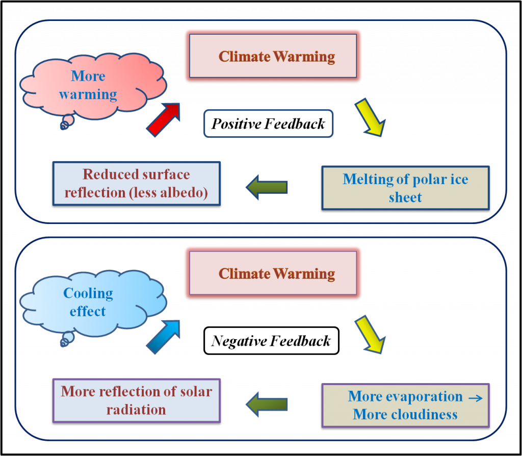
Figure 2. Examples for Positive and Negative feedback processes.
IPCC Emission Scenarios:
To standardize climate change studies, and to fine-tune policy decisions concerning climate mitigations and adaptations while targeting a mutually agreed permissible range of future climate change, IPCC has adopted a family of emission scenarios and pathways to future radiative forcings. Apart from the natural variability, future changes in climate will be dictated by the policy decisions and the level of socio-economic and technological developments. Therefore it seems suitable to project future climate variations corresponding to certain emission scenarios, which are based on a standardized set of assumptions. In line with this understanding, in the year 2000, IPCC had adopted a family of emission scenarios published in its Special Report on Emission Scenarios (SRES) (IPCC, 2000). This family of emission scenarios is called as ‘SRES’ emission scenarios.
A sequential approach had been followed in modelling future climate using SRES emission scenarios (Figure 3). IPCC realized that this approach has hindered the progress in both the areas of climate modelling (concerned with Climate Modeller (CM) communities) as well as socio-economic modelling (concerned with Integrated Assessment Modeller (IAM) communities). In a sequential approach, to project future climate, the CM community had to depend upon the narratives constructed by socio-economic models (IPCC, 2007). While during the climate modelling experiments it was cumbersome to incorporate changes into emission scenarios resulting due to the recent trend in socio-economic scenarios. Also, this approach required a great deal of coordination in sharing information between different communities, resulting in delays. Considering these drawbacks, IPCC adopted a parallel approach to future climate scenarios developments (Figure 3) using ‘Representative Concentration Pathways (RCPs)’. Suggested by the IPCC in its Expert Meeting Report of the year 2007, the RCPs talk about the trajectory of greenhouse gas concentrations and not emissions, and they are consistent with a range of scenarios of stabilization, mitigation, and emissions discussed in the scientific literature.
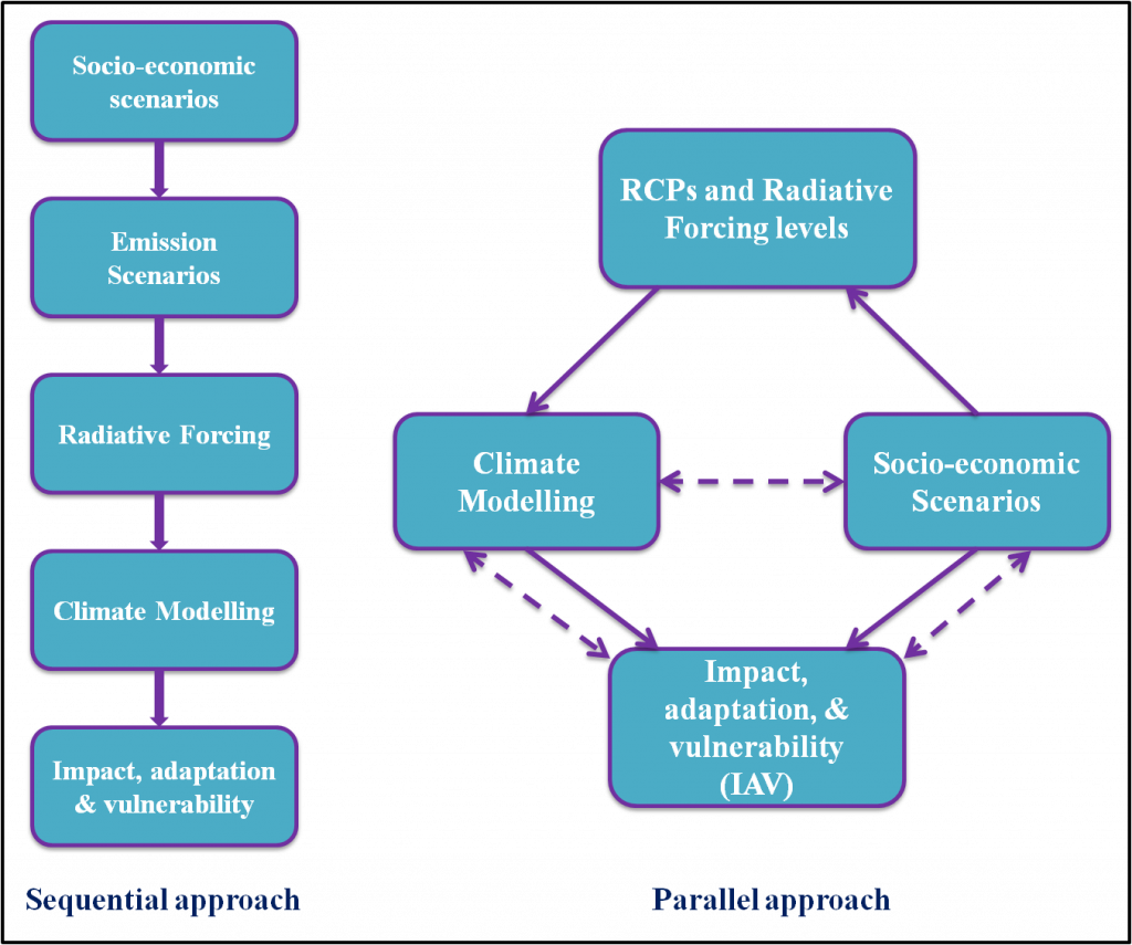
Figure 3. Two approaches to climate scenario development.
In a parallel approach, RCPs are being employed as an initial point to start making future climate scenarios, allowing climate modelling to investigate plausible projected changes in climate corresponding to various RCPs and allowing socioeconomic modelling to explore the various developmental paths to reach these RCPs. In the fifth assessment report (AR5) of IPCC, the assessed works have made use of RCPs in preparing future scenarios of climate change while superseding the use of SRES emission scenarios. A family of SRES emission scenarios and various RCPs are briefly explained below.
SRES Emission Scenarios:A1FI, A1B, A1T, A2, B1, and B2 are six SRES scenarios adopted by IPCC in its third (TAR) and fourth assessment (AR4) reports. Each scenario highlight the possible manner in which the world might develop considering different population and economic growth rates, technological advancements, and level of globalization (Table 1). Scenarios starting with letter ‘A’ show the period of more economic focus, while those starts with letter ‘B’ highlights the period of more environmental focus. The ‘1’ storylines highlight a more homogeneous global community i.e. globalization, while the ‘2’ storylines highlight a more heterogeneous global community i.e. regionalization. None of the SRES scenarios has considered the influence of future climate initiatives (such as UNFCCC or the Kyoto Protocol).
Table 1 SRES Emission Scenarios
| 1 – Globalized World | 2 – Regionalized World | |
| A (Economic interests) | Very rapid economic growth. Three groups based on technological emphasis; mid-century peak in global population & decline thereafter. A1FI – Fossil Fuel Intensive A1B – Balance across fossil & non-fossil energy sources A1T – Non fossil energy sources | Self-reliance and preservation of local identities; region oriented economic growth; continuously increasing the population. Slow & fragmented technological change & per capita economic growth. |
| B (Environmental interests) | Convergent & ecologically aware world; mid-century peak in global population and decline thereafter; a shift in economic growth towards service and information economy; use of clean and resource-efficient technologies; focus on global solutions to social, economic and environmental sustainability. | Increasing population (rate lower than A2); focus on local solutions to social, economic and environmental sustainability; intermediate level of economic growth; slow and diverse technological development compared to A1 and B1. |
Representative Concentration Pathways:
Contingent upon the ways in which GHGs will be emitted in the years to come, in its fifth assessment report, IPCC has adopted four pathways to climate futures, known as representative concentration pathways (RCPs). Scenarios selected for climate modelling and research are RCP8.5, RCP6.0, RCP4.5, and RCP2.6. Values, in the end, show the level of radiative forcing in the year 2100. The word pathway not only signifies the importance of long term GHG concentrations and corresponding radiative forcing, but also the trajectory followed to arrive at these outcomes. The word representative signifies that these pathways are representative of several different scenarios which are identical in emission and radiative forcing characteristics (IPCC, 2007). The overall procedure followed to develop these RCPs is explained in Van Vuuren et al. (2011).
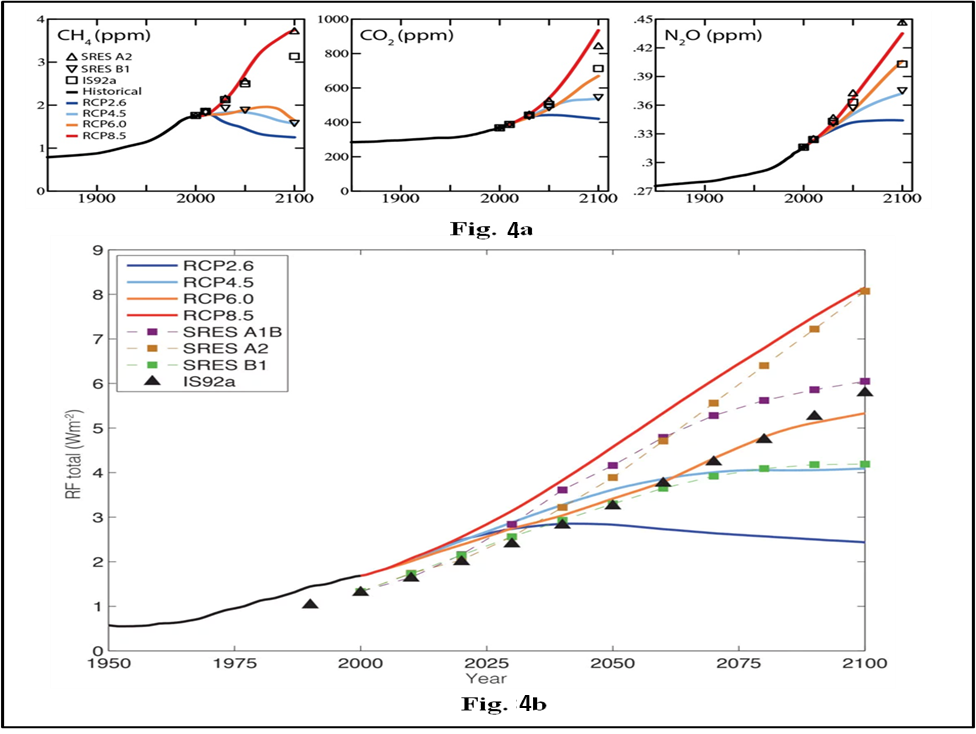
Figure 4. Evolution of GHG concentrations over time (1850-2100) (Fig. 4a); Total anthropogenic radiative forcing relative to pre-industrial times (Fig. 4b). These forcing levels do not account for forcings due to changes in surface albedo, mineral dust and nitrate aerosol. (Above graphs were obtained from IPCC’s fifth assessment report (AR5): Figure 1.15 & 8.5 (IPCC, 2013)).
Table 2 The four marker RCP scenarios (Moss et al., 2010).
| Pathway | Integrated Assessment Model (IAM) used to generate RCP | GHG Concentration (ppm) in 2100 | Radiative Forcing in 2100 |
| RCP2.6 – Peak before 2100 and then decline | IMAGE | peak at ~ 490 CO2 equivalent before 2100 & decline thereafter | peak at ~ 3 W/m2 before 2100 & decline thereafter |
| RCP4.5 – Stabilization by 2100 | GCAM | Stabilization at ~ 650 CO2 equivalent | Stabilization at ~ 4.5 W/m2 |
| RCP6.0 – Stabilization by 2100 | AIM | Stabilization at ~ 850 CO2 equivalent | Stabilization at ~ 6 W/m2 |
| RCP8.5 – Ever increasing | MESSAGE | > 1370 CO2 equivalent in 2100 | > 8.5 W/m2 in 2100 |
References
IPCC (Intergovernmental Panel on Climate Change) (2000). Chapter 4 An Overview of Scenarios, Special Report on Emission Scenarios (Working Group III of IPCC). Cambridge University Press, Cambridge, UK. https://www.ipcc.ch/site/assets/uploads/2018/03/emissions_scenarios-1.pdf
IPCC (Intergovernmental Panel on Climate Change) (2013). Climate Change 2013: The Physical Science Basis. Contribution of Working Group I to the Fifth Assessment Report of the Intergovernmental Panel on Climate Change. Cambridge University Press, Cambridge, UK. https://www.ipcc.ch/report/ar5/wg1/
IPCC Expert Meeting Report (2007, September). Technical Summary of ‘Towards new scenarios for analysis of emissions, climate change, impacts, and response strategies’.Retrieved October 15, 2019. https://www.ipcc.ch/site/assets/uploads/2018/05/expert-meeting-ts-scenarios-1-1.pdf
Kiehl, J. T., and Trenberth, KE. Earth’s Annual Global Mean Energy Budget. Bulletin of the American Meteorological Society. (1996). Vol. 78, No. 2, 197-208. http://climateknowledge.org/figures/Rood_Climate_Change_AOSS480_Documents/Kiehl_Trenberth_Radiative_Balance_BAMS_1997.pdf
Moss, R., Edmonds, J., Hibbard, K. et al. The next generation of scenarios for climate change research and assessment, Nature, 463, 747-756 (2010). DOI: https://doi.org/10.1038/nature08823.
NOAA (National Oceanic & Atmospheric Administration). (2019, October). Trends in Atmospheric Carbon Dioxide. Global Monitoring Division, Earth System Research Laboratory. Retrieved October 10, 2019. https://www.esrl.noaa.gov/gmd/ccgg/trends/
Van Vuuren, D.P., Edmonds, J., Kainuma, M. et al. (2011) The representative concentration pathways: an overview. Climate Change, 109:5-31. DOI 10.1007/s10584-011-0148-z