Climate Modelling
Why do we need to do modelling?
Scientific curiosity drives researchers across the globe to decipher the behavioural patterns of various natural systems by employing the ever-evolving tools and techniques developed using the finite scientific knowledge in hand. In some cases, various natural processes and interactions can be better understood through experimental studies. While in some cases, given the nature of complexity and the scale of a natural system, it becomes impossible to create an experimental setup. In such cases, we try to emulate natural systems using mathematical models which are compatible with the principles of physics, chemistry, and biology.
As there are many extreme climatic events, such as floods, droughts, heat-waves, and cyclones, which negatively impacts human lives, and their livelihood. Under changing climate these extreme events get intensified and become more frequent. It becomes imperative for scientists, the general public, government and non-government bodies to understand the behaviour of the climate system over a different time period, especially the future behaviour. Given the complex response of the climate system to natural and man-made forcings, it is convenient to follow a mathematical modelling approach rather than the experimental one. Climate model helps the research community to construct past and future climate state, and assist in knowing the influence of natural and anthropogenic forcings on other natural and man-made systems. Model outputs provide a rational basis for various policy decisions which are aimed at climate mitigation and adaptation. Thus, ever-evolving climate models will prove to be a game-changer in building climate-resilient cities, agriculture and water resources systems, ensuring food, water, and livelihood security of our modern society.
How do we do it?
Scientists lay the framework for climate model in line with the set ground rules which are being followed by various physical, biological, and chemical processes of the earth’s climate system (Mujumdar, 2011). Climate models can be considered to be an extension of weather models which are run over a longer time steps such as years, decades or centuries. The climate models which are used for both weather and climate forecasts are known as unified models (Met Office, 2019b). One thing to keep in mind is that the Climate models are not being used to give daily forecasts, but to give a statistically accurate picture of Climatic indicators.
Thermal energy within the earth’s system is being redistributed through the large scale circulations within oceans and atmosphere. These large scale circulations of atmospheric air and oceanic water are termed as general circulation. Climate models obey many physical and chemical laws such as the conservation of energy (the first law of thermodynamics), conservation of mass and momentum, ideal gas law, Stefan-Boltzmann law etc. In a typical climate model, these scientific principles are represented in the form of mathematical equations, which are then embedded into a computer code. Various mathematical equations help in simulating dynamic climate processes and their interaction i.e. the general circulations within the atmosphere and oceans. The most prominent mathematical equation is the Navier-Stokes equation of fluid motion which is being applied on a rotating sphere to describe various physical properties of atmospheric air and oceanic water (Scaife et al., 2007). Any typical climate model is consist of a million lines of computer code, and thus demands an enormous amount of computing power to run (Doughty-White et al., 2015). For efficient climate modelling, supercomputers are generally employed to run these models on a different space and time scales. For example, to facilitate high-performance computing in weather, climate and environmental science, the United Kingdom’s Met Office Hadley Centre had installed ‘The Cray XC40 supercomputer’ in December 2016, which is capable of performing 14,000 trillion calculations every second (Met Office, 2019a). Such enormous computing power enables it to load daily 215 billion global weather observations for running a million lines of code for an atmospheric model. Through its enhanced weather and climate forecasting, it is believed that it would facilitate £2bn of socio-economic benefits. But still, this computing power is not enough to capture climatic processes happening at every cubic meter of atmospheric volume. Therefore, to achieve computational efficiency, climate models divide the earth into a number of large grid boxes or cells (Figure 1).
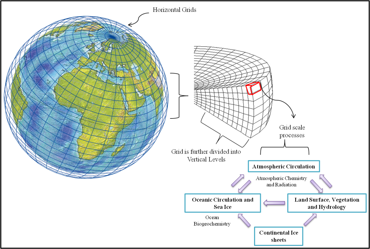
Figure 1. Graphical illustration of GCM grids.
Equations which govern the interactions and evolution of different variables during model runs are being solved at each grid cell over a predefined timestep (Carbon Brief, 2018). To simulate the climate for each grid cell during every timestep, climate model considers a single value of radiation, temperature, pressure, wind speed, and humidity for that cell. Model output at the grid point does not represent the real-world value; rather it can be taken as a mean value for that particular grid cell. Sometimes due to the complexity of a process involved, it becomes difficult to explain it with a limited scientific understanding, such as the process of cloud formation. For such complex processes and the processes happening at smaller scales than the grid size, climate modellers take resort of ‘parameterization’. Process of the parameterization facilitates the approximate representation of these processes into a climate model. But, due to such simplifications, we have to compromise with the accuracy of climate model outputs.
In short, various processes gets evolved during model runs, enabling the climate model to decide everything like oceanic currents, moisture fluxes, seasonal climate cycles, the direction of a wind, the location of rainfall, and the carbon cycle (Schmidt, 2014).
How did Climate Models evolve overtime?
Medieval era Ocean expeditions had helped humans to understand wind patterns reflecting from the large scale atmospheric circulations. Sailors started plotting wind directions to prepare expedition maps. But all such expeditions resulted only into the understanding of the regional wind patterns. It took to until the 18th Century for someone to come up with scientific explanations of these wind patterns on a global scale. In 1735, an English amateur meteorologist George Hadley explained the presence of trade winds (easterly flows) using the law of conservation of angular momentum (Harper, 2007). These trade winds are also known as Hadley circulation. In the 19th century, a simplified three-cell model of global-scale atmospheric circulation was put forth by American meteorologists William Ferrel and James Coffin. Still, the scientific understanding was limited to the surface phenomenon due to lack of observations in upper layers of the atmosphere.
In the early 20th century, the British Meteorologist David Burnt emphasised on the importance of understanding temperature variability and corresponding pressure patterns to draw conclusions on wind patterns. In the second half of the 20th century, the use of numerical weather prediction techniques and advances in computer applications had helped meteorologist to start developing climate models. In 1956, an American Meteorologist Norman Phillips developed an atmospheric model simulating a general circulation over a regional scale with predefined initial conditions and produced outputs for 31 days in advance. His model was incapable of distinguishing in-between land and oceans, but it became the basis for the development of atmosphere-only models to today’s complex Earth system models. Integration of atmosphere-only and ocean-only models into a coupled atmosphere-ocean general circulation models (AOGCMs) is regarded as a significant development in the area of climate modelling. Process of developing several other components separately and then integrating them into a climate model is still in progress (Figure 2).
In the recent state of the art climate models the various components which are being integrated are:
- atmosphere
- land surface and carbon cycle
- ocean and sea ice
- aerosols (sulphate and non-sulphate)
- dynamic vegetation
- atmospheric chemistry
- land ice
- ocean biogeochemistry
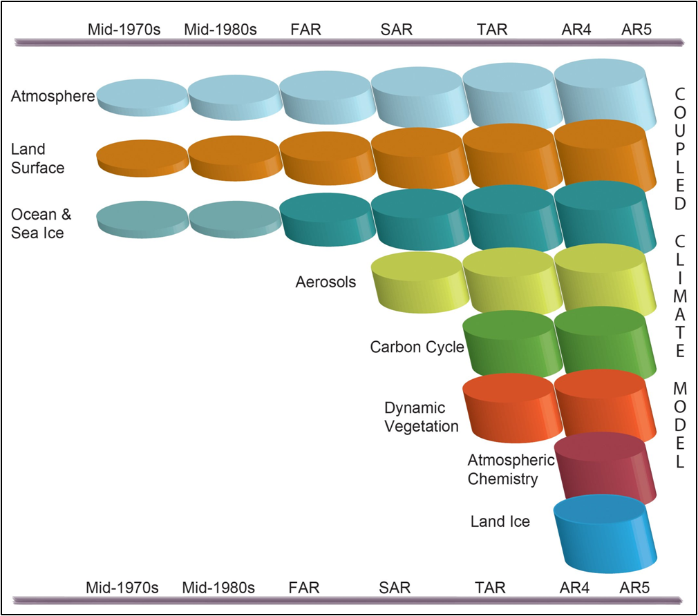
Figure 2. Evolution of Climate Models over time with increased complexity and inclusion of new components (IPCC AR5 (2013): WG1, Chapter 1, Figure 1.13; https://www.ipcc.ch/report/ar5/wg1).
GCM & RCM:
Climate modelling is one of those research domains which require extensive computational power. A grid size of a climate model defines its spatial resolution, and the temporal resolution tells how frequently model creates the state of the climate system i.e. the timestep. Due to the limitations in computational efficiency, these two types of model resolutions are not independent of each other (UCAR, 2019). In order to create a three-dimensional numerical model, the earth’s surface is being divided into a horizontal grid, and atmosphere and ocean into vertical levels and calculations are done in discrete timesteps. To have a computationally efficient model run over the entire globe, these models are divided into coarsely spaced horizontal cells (generally, in between 200 to 100 km) (Figure 3). These models are known as General Circulation Models (GCMs) or Global Climate Models (GCMs). The processes happening at the sub-grid scales are either parameterised or ignored (Raje et al., 2013). In climate change impact studies, this affects the accuracy of hydrologic variables (precipitation, temperature, runoff, evapotranspiration) simulated based on GCM outputs. GCMs don’t account for orography, islands, land use, coastlines, and vegetation dynamics at a scale smaller than the grid size. Thus, GCMs are suitable only to define a state of global climate by factoring into the effects of global greenhouse gas emissions, volcanic eruptions etc. They may produce fairly well results of local climate over topographically more uniform hinterlands or over the vast ocean expanses.
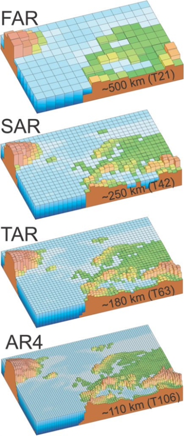
Figure 3. Increasing GCM resolution in successive IPCC assessment reports. (IPCC AR4 (2007): WG1, Chapter1, Figure 1.4; https://www.ipcc.ch/site/assets/uploads/2018/03/ar4-wg1-chapter1.pdf).
In order to assess the impact of climate change on local natural and manmade systems, one can’t rely on coarse-scale GCM outputs. For example to estimate the state of local water resources after a few decades under changing climate scenario, one needs model outputs at a much finer resolution. For this purpose, climate scientists employ various downscaling techniques. Downscaling is a term used to explain the process of predicting local scale climate variable by factoring into the large scale climatic variable obtained from GCM output. In general downscaling techniques are being grouped into two major classes: Statistical Downscaling (SD), and Dynamical Downscaling. Under Statistical downscaling methods, regression models are being developed to establish a statistical or empirical relationship between GCM outputs (predictors) and a local climate variable (predictand). Efficacy of these regression models depends upon the quality of data used for calibration. Dynamical downscaling techniques employ high-resolution regional climate models (RCMs) (Figure 4). Compared with GCMs, RCMs simulate the climate at a finer resolution (around 25km or less), but for a limited area in order to have a computationally efficient model runs (climateprediction.net, 2019b).
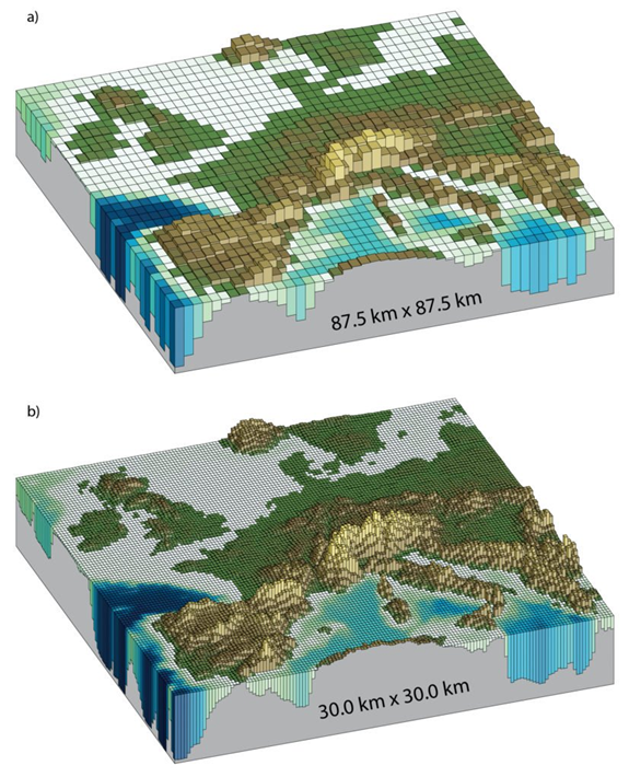
Figure 4. Topographic details get improved with increase in model resolution ; Fig. 4a & 4b shows representation of European topography with 87.5 X 87.5 km grid (resolution of recent GCMs) & with 30 X 30 km (resolution of regional models). (IPCC AR5 (2013): WG1, Chapter 1, Figure 1.14; https://www.ipcc.ch/report/ar5/wg1).
Over limited spatial domains, RCMs solves the governing equations of atmospheric and oceanic dynamics by incorporating values supplied at their boundaries either from the observed data or from the GCM output. In order to ensure a continuous supply of data at RCM boundaries, usually, RCMs are run nested within the global climate models. Based on the nature of information supply in between RCM and GCM, there can be either one-way or two-way nesting. Although one-way nesting is computationally more efficient, two-way nesting is considered to be a more accurate way of using RCMs. In two-way nesting, information produced from the RCM outputs is being supplied back to the GCM.
Advantages of RCMs over global models can be summarized as follows:
- Detailed prediction of climate change: as it accounts for topography and other local factors; its results might be in contradiction with the GCM results at local scale.
- Resolution of smaller islands.
- Prediction of variations in weather extremes: GCM outputs emphasise on changes in long-term climate statistics, but the knowledge of extreme weather events is more important to build climate resilience.
- Simulation of cyclones or hurricanes: as the intensity and frequency of cyclones would get altered by climate change, RCMs are more suitable to resolve cyclonic events at finer scales.
- Use of RCM outputs for impacts studies: for example, RCM output on precipitation and temperature can serve as an input for hydrological models or urban flood models.
Model Ensembles:
Although climate modelling approach is considered to be a reasonable way of defining the state of climate for different space and time scales, the climate model outputs can’t be taken for granted as a basis for assessment, mitigation and negotiations. No climate model is perfect in simulating various climate features. Model imperfection or uncertainty in prediction stems from varied factors such as parameterization, structural flaws, missing local details, and boundary conditions. To address such uncertainty climate modellers employ model ensembles i.e. to understand the average climate behaviour from different runs of a single model under varied conditions or multi-model runs. Every climate model in these ensembles has slightly different features producing different outputs. Two types of ensembles mentioned by the IPCC in its assessment report are as follows (IPCC, 2013):
- Multi-model ensembles (MMEs)
Such ensembles comprise of independent models from different climate modelling centres. They are employed to test the model structural uncertainty and internal variability. As many models around the world have been developed with shared components, the number of independent models is small. Therefore, to avoid a shared bias, model size of these ensembles is kept small. - Perturbed-parameter ensembles (PPEs)
Due to limited computing power and scientific understanding, some sub-grid scale processes are parameterized and their values are adjusted empirically to fit model outputs to observed data. This leads to uncertainty in model outputs. Therefore, PPEs are used to understand the effect of a plausible range of these parameters on single model output. This approach helps in short-listing such parameters to which model outputs are more sensitive. But it can’t be employed to assess model structural imperfections. Sometimes, these ensembles are also known as Perturbed Physics Ensembles, because the parameters which control the physical processes in models are being perturbed. Here, each model could be considered unique, as each of them is having a different set of parameters.
Some studies follow a combination of both of these approaches. While some climate experiments suggest two additional approaches (climateprediction.net, 2019a):
- Initial Condition Ensembles
In such an ensemble, a single model (i.e. for same atmospheric physics) evolution is being studied by having thousands of model runs with a different start date. These ensembles help to decipher the internal variability of the climate system. With this ensemble, a climate model driven with known forcing conditions can be validated against observed data i.e. by hindcast. These ensembles also used to find such processes within the climate system which are sensitive to initial conditions. - Forcing Ensembles
These ensembles help to assess model sensitivity to varying forcing conditions. Sometimes, this approach is also used to separate the influence of any typical forcing on model outputs, to understand its effect by comparing future projections with current simulations.
Except for multi-model ensembles, all other ensembles sample a range of single model outputs. It is also possible for a model to have a bias or yield a systematic error. In such cases using multi-model ensemble is considered to be a suitable approach than having a single model ensemble. Because it may reduce the resultant error by balancing out the bias originating from different models.
References
Scaife, A., et al. (2007). A model approach to climate change. Physics World. 20 (2), IOP Science. https://doi.org/10.1088/2058-7058/20/2/29
Carbon Brief (2018, January). Q&A: How do climate models work? Carbon Brief Limited, UK. Retrieved November 21, 2019. https://www.carbonbrief.org/qa-how-do-climate-models-work
climateprediction.net (2014, July). Climate Ensembles. Climate Experiment by University of Oxford, UK. Retreived November 21, 2019. https://www.climateprediction.net/climate-science/climate-ensembles/
climateprediction.net (2019, June). Regional Climate Models. Climate Experiment by University of Oxford, UK. Retreived November 21, 2019. https://www.climateprediction.net/climate-science/climate-modelling/regional-models/
Doughty-White, P., Quick, M., and McCandles, D. (2015). Codebases: Millions of lines of code. informationisbeautiful.net. Retreived November 18, 2019. https://informationisbeautiful.net/visualizations/million-lines-of-code/
Harper, K. (2007). ‘Weather and climate: decade by decade’. Facts on File, US. 1st edition. ISBN 13: 9780816055357.
IPCC (Intergovernmental Panel on Climate Change) (2013). Chapter 9- Evaluation of Climate Models, in Climate Change 2013: The Physical Science Basis. Contribution of Working Group I to the Fifth Assessment Report of the Intergovernmental Panel on Climate Change. Cambridge University Press, Cambridge, UK. https://www.ipcc.ch/report/ar5/wg1/
Met Office, UK. (2019). The Cray XC40 supercomputer. Retrieved November 19, 2019. https://www.metoffice.gov.uk/about-us/what/technology/supercomputer
Met Office, UK. (2019). Unified Model. Retrieved November 20, 2019. https://www.metoffice.gov.uk/research/approach/modelling-systems/unified-model/index
Mujumdar, P. P. (2011). ‘Implications of Climate Change for Water Resources Management’, India Infrastructure Report. Chapter-2, pp. 18-28. Oxford University Press.
Raje, D., Ghosh, S., and Mujumdar, P. (2013). Book chapter- Hydrologic Impacts of Climate Change: Quantification of Uncertainties. Climate Change Modelling, Mitigation, and Adaptation, edited by Rao Y. Surampalli et al. American Society of Civil Engineers, United States. ISBN: 978-0-7844-1271-8.
Schmidt, G. (2014, March). The Emergent Patterns of Climate Change. TED Talk. Retreived November 22, 2019. https://www.ted.com/talks/gavin_schmidt_the_emergent_patterns_of_climate_change
UCAR (University Corporation for Atmospheric Research), Center for Science Education. Climate Modelling. Retreived November 20, 2019. https://scied.ucar.edu/longcontent/climate-modeling
Related links
https://youtu.be/toCFqOGVs54 – Video on Climate Modelling created by the Commonwealth Scientific and Industrial Research Organization (CSIRO) in collaboration with the Australian Bureau of Meteorology.
https://www.gfdl.noaa.gov/climate-modeling/ – Climate Modelling, Geophysical Fluid Dynamics Laboratory, NOAA, US.
https://oxfordre.com/climatescience/view/10.1093/acrefore/9780190228620.001.0001/acrefore-9780190228620-e-27 – Downscaling Climate Information, Rasmus Benestad (2016), Climate Science, Oxford Research Encyclopedia, Oxford University Press, USA.
https://esgf-node.llnl.gov/projects/cmip5/ – Coupled Model Intercomparison Project 5 (CMIP 5).